Ray tracing is a way of rendering an image by simulating light propagation as it happens in the real world. Each light source generates an infinite number of light rays, that go in various directions. When one of those light rays hits the surface of a (non transparent) object, it gets diffused and some of it’s colors are “filtered”, depending on the object’s color. When one of those diffused rays hits the observer’s eye, that observer sees the object in the colors that were not filtered out by that object.
The goal of ray tracing is to determine, for each pixel on the rendering screen, the color it would have by doing some kind of backward analysis : start a ray for each pixel, called view-ray, and test if that view-ray hits any object. If it does, look if that intersection point is illuminated by any light source, and if it is, find it, and set the color of the pixel according to the combination of light source-color and object-color. That way, one can simulate any kind of lighting (totally white as well as fire red) for any kind of colored object. It is also possible to simulate nice-looking visual effects such as transparency, blur, or reflection. In fact, for reflection, which is implemented in the example, one simply needs to add to the already computed color component another component, the reflection component, which is determined by again doing ray tracing where you take the object that has the reflecting surface as an observer. Indeed, the reflection on an object’s surface is like asking “what does the object see?”.
This technique, even though it produces really beautiful results, can not be used for real time applications, since it requires an enormous amount
of calculations. For each pixel, one must create a ray, test this ray for intersection with every object, and after an intersection has been found, test
this pre-diffused ray for an intersection with every light-source. Adding reflection to that makes it even more computationally expensive.
So in most real-time applications such as games, other rendering techniques using approximations, such as rasterization are being used. However, ray tracing is used a lot to render 3D-animation movies,
as well as to beautify pictures. Because each pixel can be rendered independently from the others, ray tracing can be trivially parallelized by simply computing
each pixel independently, and assigning each available core some pixels to render.
For that, we need a Scheduler that will execute our rendering operations in parallel.
In order to do that, we first create a default scheduler configuration conf that specifies the number of cores we want to use.
Then, we can instantiate our scheduler using that configuration. Now we can simply call .toPar on our Range and that’s it.
val img = new BufferedImage(Witdth, Height, BufferedImage.TYPE_INT_ARGB)
val conf = new Scheduler.Config.Default(numberOfCores)
implicit val s = new Scheduler.ForkJoin(conf)
for (pixel<- ((0 to Witdth*Height -1).toPar))  {
  val y  = (pixel / Witdth)
  val x  = pixel % Witdth
  img.setRGB(x, y, drawPixel(objects, lights, zoom, reflectionRate, x, y))
}
s.pool.shutdown()
img
We used the default workstealing tree scheduler for this example. Notice that our code is slightly different because we do not want to create a new scheduler each time we draw a new image.
1) Representing the image
First, we need to define how exactly those camera-rays are being created. For that, we need to have a representation of the screen that our rays have to traverse. In the case of the example application, this is a 640 x 480 pixel grid. Now one very simple possibility is to make each camera-ray start at a different pixel, and give it a direction perpendicular to the screen grid.
This, however, does not create a physically accurate image : each pixel has been “seen” from a different point of view, so the relative positions of the objects are not accurate. And when one tries to change the part of the scene that is being looked at, those relative positions do matter a lot. Moreover, this does not represent what we intuitively think of a “camera” : there should be only one starting point for all the view rays, and that is where the camera is located. Hence one has to adjust the directions of the rays such that each ray goes through it’s corresponding pixel.
This can be done by computing for each pixel, it’s coordinate in the world. By convention (and also to make things simple), the camera is placed exactly one unit in z-direction behind the rendering screen, where all pixels are. So we already know that each pixel’s z-coordinate is simply the camera’s z coordinate + 1, so the z-component of the direction vector is simply 1.
We choose to represent the rendering screen by a 2 x 2 screen, where the middle is located directly one unit in z-direction away from the camera. A detailed tutorial about how to construct a rendering screen can be found here.
To get the formulas for each direction, we can consider to move camera and screen to a position that makes it easier for us to think about it, and worry about the offset later. For example, the screen’s central point can be located in (0,0,0), whereas the camera is located in (0,0,-1). We want to get each (x,y) coordinate of pixels that varies 0 to 640, respectively from 0 to 480 to now vary between -1 and 1. Let’s focus on the x-coordinate. By dividing x by 640, we get a number between 0 and 1. Multiplying it by 2 and subtracting 1 yields us a number between -1 and 1.
By doing this in both directions we get the following pixel coordinates :
val xx = (2 * (x.toDouble / WIDTH.toDouble) - 1)
val yy = (1 - 2 * (y.toDouble / HEIGHT.toDouble))
Now, since we said that our camera was located on (0,0,1), and the screen in (0,0,0), the vectors from the camera to those pixels are directly (xx,yy,1), which will be our direction vectors for our camera rays. We also need to multiply one of those coordinates by the aspect ratio of the image to account for the fact that the pixels of the image are not square. Finally, one can easily add a zoom factor representing how much of that image is being rendered.
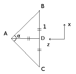
Let α be the angle that represents how much of the image plane BC is being seen. We can see that tan(α/2) = BD/AD. Since we said that the camera is always one unit always from the screen, AD will always be 1. Hence BD = tan(α/2). BD represents how much of our image is being rendered in x-direction. In the particular case of our image, without any zooming in, α = π/2 and BD = 1. We can draw the same figure for the y-z plane and obtain the same result : hence we must multiply both expressions by tan(α/2) in order to have a zoom. In Scala, this becomes :
zoomFactor = Math.tan(Math.PI * 0.5 * α / 180)
where zoom is an angle in degrees between 0 and 90. We just converted the angle from degree to radian.
Hence, our final expressions for the camera-ray directions are :
val xDirection = xx * aspectratio * zoomFactor
val yDirection = yy * zoomFactor
val zDirection = 1
Now we that we know each camera-ray’s starting point and it’s direction, we can actually start the tracing part of our raytracer.
2) Intersections and Rays
First, let us introduce the different kinds of objects needed for our raytracer.
Our most used object is a 3-dimensional-vector. We need it for Rays and Colors.
class Vector3(xt: Double, yt: Double, zt: Double){
  var x: Double = xt
  var y: Double = yt
  var z: Double= zt
  val squareNorm = scalarProdWith(this)

  def subtractVector(v2: Vector3): Vector3
  def scalarProdWith(v2: Vector3): Double
  def crossProdWith(v2: Vector3): Vector3
  def normalize(): Vector3
}
In our Ray-class, we store the variable t computed during our intersection-testing function. It represents up to how far from the starting point we consider the ray (this makes the intersection computation faster). If an intersection was found, we only consider the ray up to that intersecting point, which can be calculated by computing start + t·dir.
class Ray(rStart: Vector3, rDir: Vector3, rT : Double) {
  var start : Vector3 = rStart
  var dir = rDir
  var t : Double = rT
}
The Material class defines the color of the objects as well has how much they reflect the light.
class Material(colorS : Vector3, reflectionS : Double){
  val color : Vector3 = colorS
  val reflection : Double = reflectionS
}
And of course, we need the objects we want to render.
abstract class RenderObject(mat: Material){
  val EPSILON = 0.000001
  val material = mat

  def intersect(r: Ray): Boolean
  def normalVectorToSurfaceAtPoint(point: Vector3): Vector3
}

class Sphere(sPos: Vector3, sSize: Double, mat: Material)
  extends RenderObject(mat: Material) {

  val center: Vector3 = sPos
  val radius: Double = sSize

  def normalVectorToSurfaceAtPoint(point: Vector3): Vector3
  def intersect(r: Ray): Boolean
}

class Light(lPos: Vector3, lcolor: Vector3) {
  val pos : Vector3 = lPos
  val color = lcolor
}
As pointed in the introduction, the part of our program that we will be used the most is the intersection verification part.
For that, we need to be able to compute the intersection between a line and our objects.
In the case of a sphere, we can simply take the sphere’s equation and the line’s equation and solve for the unknown that makes them both be equal. We then get a quadratic equation determining the intersections of that sphere with that line. Here is a how this can be implemented :
def intersect(r: Ray): Boolean = {

  val A = r.dir.scalarProdWith(r.dir)
  val diffRaySphere = r.start.subtractVector(sphere.center)
  val B = 2 * diffRaySphere.scalarProdWith(r.dir)
  val C = diffRaySphere.scalarProdWith(diffRaySphere)-radius*radius
  val delta = B*B - 4* A*C

  if (delta <0){
    return false
  }
  val t0 = (-B - Math.sqrt(delta))/(2*A)

  //take the first intersection with the sphere.
  if (t0 <= r.t && t0 > EPSILON){
    r.t = t0
    return true
  }
  //compute t1 only if necessary, as we allways have t0<t1
  val t1 = (-B + Math.sqrt(delta))/(2*A)
  if (t1 <= r.t && t1 > EPSILON){
    r.t= t1
    return true
  }
  return false

}
But, as this portion of code is used really often (ImageHeight*ImageWidth*(NumberOfSpheres + NumberOfSpheres*NumberOfLights)*ReflectionRate) times in the worst case,
we must really try to be as efficient as possible. This involves not recreating any Vector3-object within this function, which makes it a little bit
less readable, but also faster. When the number of spheres gets large as in the spherePool-setting, the difference can be in the tens of milliseconds.
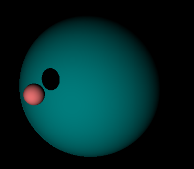
One might wonder why we test t0 > 0.0001. This is to avoid imprecision errors. If we write instead t0 > 0, we get artifacts :
The line-sphere equation can have two solutions, as it is quadratic, but we only consider the first intersection encountered by the ray on it’s traversal.
In order to see why, let us explain how our raytracer works :
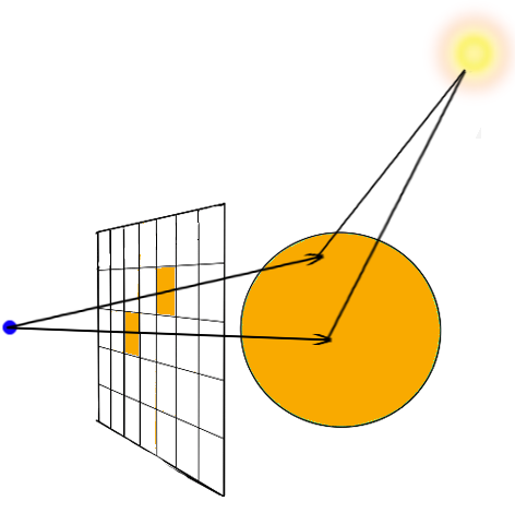
Our goal is to find out the correct color for pixel p. We know it’s coordinates on the screen and have it’s corresponding camera-ray.
Now, the first thing we do is testing if our camera-ray hits a sphere, i.e. if we could be able to see it given our current position and the position of the sphere. This is the first case for which we need our intersection method. Remember that our camera ray starts at the camera and traverses the screen, and our camera will see the side of the sphere that is the closest to it, which is determined by the intersection having the smallest t-value. We do not care about the other intersection : we can never see that side of the sphere from this point of view.
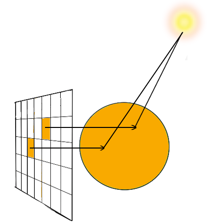
The second case arises right afterwards. That is, now that we have found an intersection point I on sphere S, we must see if there is a light that illuminates it. For that, one can simply go through the collection of all lights, and compute for each the corresponding vector between I and that light. Each of those light rays might contribute to the final color of p. But not every light does. Only the light rays that do not have any obstacle in their way from I to the light will contribute.
All that we have to do is to, again, check for an intersection between our light ray and an object. For that, we must go through the collection of all objects and test each of them for intersection with the light ray. This time, we do not care where the intersection point is : we only want to know if an intersection was found. If that’s the case, we know that I is does not receive any light from that light source. If we went through all the light sources and allways found an intersection, then I is in the shadow of some object.
All that is left to do is to sum up all contributions of light that I received, and filter them according to the natural color of S. This works as follows :
if(!inShadow) {
  val lambertValue = lightRay.dir.scalarProdWith(n) * reflectionCoefficient
  red += lambertValue * currentLight.color.x*currentObject.material.color.x
  green += lambertValue * currentLight.color.y*currentObject.material.color.y
  blue += lambertValue * currentLight.color.z*currentObject.material.color.z
}
For each color component (red, green, or blue) the color intensity added corresponds to the intensity cast out from the light source, multiplied by the absorption factor of the material of the current object for this component (which can be between 0 and 1). 0 means that the material does not diffuse any of the light, it absorbs it all, and 1 means it diffuses it all. For example, a sphere with the material that has as diffusion Vector (1,1,1) will be completely white when illuminated by white light.
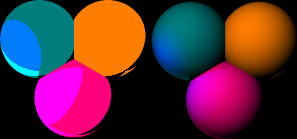
Now what about this lambertValue? This value comes from Lambert’s cosine Law. This law describes how the intensity of light diffusion on the surface of an object varies with the angle on how that light hits the surface. Intuitively, this means that if the light ray hits the object-surface with an angle perpendicular to it’s surface, that object will diffuse much more of that light as if it the light ray came from an angle almost parallel to it’s surface. As you might have guessed, if that angle is parallel, then the object diffuses no light. Lambert’s cosine Law states that the diffusion intensity is directly proportional to the cosine of the angle between the light ray and the normal vector n to the object’s surface. So we just compute the scalar product of the light ray and n to get that value. In the end, we need to take the absolute value of that cosine because we do not want to end up subtracting light : we want the Lambert-coefficient to stay between 0 and 1. The results of applying this law on spheres is quite impressive : on the left you see the scene rendered without applying Lambert’s cosine law, and on the right with it.
Now, all that is left to do is the reflection-part of our algorithm. For this, one must simply notice that the reflection on an object’s surface is simply what that object would see if it was a camera (like when you look in a mirror). So we just need to run another instance of our ray tracing algorithm, starting with a new camera-ray, which starting point will be I. It’s direction, as stated by the laws of reflection in physics, is determined by the following property : the angle of the reflection-camera-ray with respect to the normal to the object is the opposite of the angle between the camera ray with respect to the normal.
By doing the math, one arrives at the following result for our new camera-ray (instantiated as a new Ray) :
val reflection =  2*currentViewRay.dir.scalarProdWith(n)
val reflectionRayDirection = currentViewRay.dir.subtractVector(
  new Vector3(n.x*reflection, n.y*reflection, n.z*reflection))

computeColorContribution(new Ray(intersectionPoint, reflectionRayDirection,
  MaxLengthRay),
  reflectionLevel+1,
  reflectionCoefficient*currentRenderObject.material.reflection)
The method computeColorContribution computes the color contribution for a given camera ray : first, it is called for our actual camera ray,
and then it calls itself for each reflection.
The reflection-process can be repeated multiple times. In our program, we decided to reflect each surface two times.
The value currentRenderObject.material.reflection, which ranges between 0 and 1, determines by how much the intensity of the reflected rays
decreases at each iteration.
The code of this part of the program is located in the drawPixel method.
Finally, our ray tracer is not limited to spheres. It can also render general polygonal objects by being able to render triangles.
For that, all that needs to be done is to create another class that extends RenderObject, and to redefine the intersect method, so that it
now computes the closest intersection between a ray and a triangle.
class Triangle(xT: Vector3, yT: Vector3, zT: Vector3, mat: Material)
  extends RenderObject(mat: Material){

  val x = xT
  val y = yT
  val z = zT
  val e1 = this.y.subtractVector(this.x)
  val e2 = this.z.subtractVector(this.x)

  def normalVectorToSurfaceAtPoint(point: Vector3): Vector3
  def intersect(ray: Ray): Boolean
}
We chose to use a slightly modified version of the Möller–Trumbore ray-triangle intersection algorithm for that.
This is how it looks like in Scala :
def intersect(ray: Ray): Boolean = {
  //Find vectors for two edges sharing V1
  val P = ray.dir.crossProdWith(e2)

  //if the determinant is near zero, then the ray lies in plane of triangle
  val det: Double = e1.scalarProdWith(P)

  if (det > -EPSILON && det < EPSILON){
    return false
  }
  val inv_det = 1 / det
  val T = ray.start.subtractVector(this.x)
  val u = T.scalarProdWith(P) * inv_det

  //The intersection lies outside of the triangle
  if (u < 0 || u > 1){
    return false
  }
  val q = T.crossProdWith(e1)
  val v = ray.dir.scalarProdWith(q) * inv_det

  //The intersection lies outside of the triangle
  if (v < 0 || u + v  > 1) {
    return false
  }
  val t = e2.scalarProdWith(q) * inv_det

  if (t <= ray.t && t >EPSILON) {
    ray.t = t
    return true
  }
  return false
}
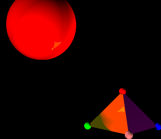
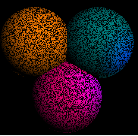
Again, as with the spheres, we can save some computation time by not creating Vector3 objects in this calculation. The result is less readable, but faster code. Now, we can construct shapes with our triangles : in the app, we have two examples showing a tetrahedron.
3) Camera movement and angles.
Now that we can render an image, it is time to look at how we can move around in the scene. To make the camera move is quite simple : as all camera rays start at the camera, we simply need to move the starting points of each camera-ray to the new position of the camera.
What’s harder is to rotate the camera in all directions. For this, we need to introduce two angles : p (pitch), which makes the camera rotate up or down, and j (yaw), which makes it rotate left or right. What we need to define is the direction in which the camera looks, which is the z-axis for the camera. We will store this information in a vector called M. More precisely, M is the unit vector from the camera to the central point of the image. It is the camera’s z-axis. Moreover, we will define the screen plane by two perpendicular unit vectors, Nx and Ny, standing for the camera’s x-axis, and the camera’s y-axis, respectively.
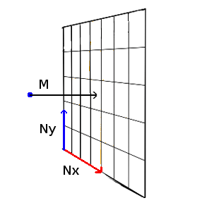
The blue point is where the camera is located. M has a direct influence on the image that is rendered : if the camera looks up, the image that is seen must also be moved up and rotated appropriately. Recall that the camera is allways located exactly one unit away in z-direction from the image. Moreover, the image-screen is allways perpendicular to M. This means that the three vectors M, Nx and Ny must be perpendicular at all times. Indeed, if that is not the case, we would see “distorted” objects. It’s exactly like when you read a piece of paper : in general, your eye is perpendicular to the paper. If you turn the paper, what can be seen on it appears distorted. Now how do we find those 3 vectors? First, notice that once we have found two of them, the third can directly be computed with a cross product between the other two. This leaves 2 vectors. Let’s start with M. When only p varies, the only thing that changes are M’s y and z components. When p is 0, we want to see the same thing as without angles, i.e M = (0,0,1). When p increases, M’s y-component increases whereas M’s z-component decreases. When we rotate the camera upwards with p = π/2, we want to have M = (0,1,0) : the camera should look up. As this is supposed to repeat itself modulo 2π, we can see that our provisional M = (0, sin(p), cos(p)). Now what happens, if, given p, we change j ? For that, let’s look at this situation in the x-z plane, from the top. When j increases, we rotate to the left, in -x direction, and move away from our maximum z.
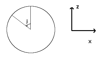
By looking at the trigonometric circle drawn in the figure, we see that we add a component of -sin(j) in the x-direction and cos(j) in the z-direction. The y-direction is unchanged.
Thus our final vector is M = (-cos(p)sin(j), sin(p), cos(p)cos(j)), which has norm of 1. Now let us consider Nx, the vector representing how the image is turned in x-direction depending on the p and j. Since Nx must be perpendicular to M, we know that Nx lies in the plane perpendicular to M. As a vector in a plane is defined by two dimensions, we can set one of Nx’s entries to 0. We chose the y-entry, as this has the realistic-seaming effect of not making the camera roll over while it turns (if we would watch the skyline with our camera, it would allways be horizontal). So we must only orient that vector in this plane, and this can be done with one angle. As we chose j to be the angle that makes the camera turn from left to right, and as Nx defines the direction of “left or right” with respect to the camera, we say that it only depends on j. Since we want Nx to be a unit-vector, one entry can be cos(j) and the other sin(j). We pick the combination that makes the scalar product M·Nx = 0.
It is : Nx = (cos(j), 0, sin(j)). Now Ny = M x Nx = (sin(p)sin(j), cos(p), -sin(p)cos(j)). A quick calculation verifies that Ny is also a unit vector.
Now we can orient the camera ray according to our camera’s coordinate-system defined by M, Nx and Ny. Hence, a pixel with normalized coordinates xx and yy on the screen will have a camera-ray with the following direction associated with it :
M + xx·Nx + yy·Ny. In our scala code, this becomes :
val xDir = -cosPitch*sinYaw + xx*cosYaw + yy*sinPitch*sinYaw
val yDir = sinPitch +yy*cosPitch
val zDir = cosPitch*cosYaw  + xx*sinYaw - yy*sinPitch*cosYaw
Now we can truly explore the scene in 3D! One last thing to add is to move in the camera’s coordinate system, and not in the overall world-coordinate system. For now, if we turn with a pitch of π/2 up and try to move forward, we will move forward in world coordinates, which will look like moving up for us. An easy way to change that is to multiply every change in a certain direction with it’s corresponding camera-direction-vector. So, a change c in y-direction will make a change of c·Ny in the overall direction of the camera. It’s the same for a change in x-direction where we make a change of c·Nx and a change on z-direction where we make a change of c·M. In the code, we have the following, where calculation represents the amount of change on the y-axis :
xOff += calculation*sinPitch*sinYaw
yOff += calculation*cosPitch
zOff -= calculation*sinPitch*cosYaw
The parts where x and y coordinates change is located in the MouseMotionListener that is added to the class RenderImage, and the part where z-coordinates and the angles change is located in the KeyListener that is added to it.
You can see the complete code for the Parallel Ray tracer here. If your browser supports Java, you can also run the applet below directly to explore the different scenes that you can choose from, and compare the performance of the classic parallel collections with the performance of the new scheduler.